Background
Back in 2022, Candia et al. [1] put out a nice study in Scientific Reports diving deep into preprocessing SomaScan datasets. Alongside their paper, they released a repository of anonymized raw and processed data with code for each step in their pipeline. This is an invaluable resource to get a handle on working with SomaScan data and discussing QC.
One of the cool things about the design in this dataset is that there are multiple types of samples with different purposes. In addition to 1704 experimental samples, the dataset contains pooled experiment “calibrator” samples and “qc” samples supplied by SomaLogic. There is also a series of “buffer” samples which can be used to assess limits of detection.
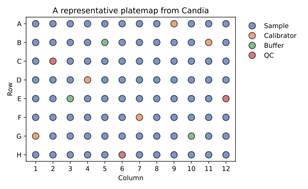
The calibrators were used extensively in the paper for data normalization, making them a bit suspect for calculating the coefficient of variation (CV). So the authors used 102 experiment samples which had 2 technical replicates in the experiment to show reduction in CV with processing steps. In this post, I will talk about how the authors calculated CV for these, why they used replicated samples, and a more straightforward alternative method for CV calculation.
Classic CV calculation
The classic definition of CV is just $$ \frac{s_n}{\bar{x}_n}$$ where $s_n$ is that sample standard deviation and $\bar{x}_n$ is the sample mean. This works fine for things like the pooled calibrator samples but breaks down for true patient samples. Patient samples are overdispersed, since measurements theoretically represent patient variation and the cumulative history of the sample since it was drawn. The technical noise from the assay is only small portion of this variation. Check out how dramatic the difference can be between the pooled and patient samples below.
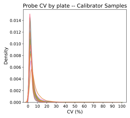
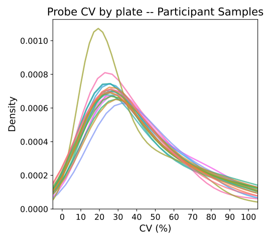
For the calibrator samples, median plate CVs range from 2.41% to 5.38%, which fits well within the expected CVs compiled by SomaLogic. On the other hand, median plate CVs for patient samples range from 26.1% to 38.2%.
CV on paired samples (Candia et al.’s method)
Measurement variation in samples from the same individual represent all the sources of variation since the samples were split. If we have two aliquots from the same blood draw, the variation represents the whole sample prep process. If two plate wells were filled using the same source, then the variation represents assay variability.
In the Candia et al. dataset, there are a series of 102 samples with 2 technical replicates. Instead of looking at sample by sample variation, the authors look at the fold change between the two replicates (with the max measurement divided by the min measurement). They note that a 2002 article by Reed et al. [2] gives an expression for the theoretical number of these fold changes greater than a factor k.
$$ P(\max \{\frac{Y}{X}, \frac{X}{Y}\} \ge k) = 2\Phi \left[ \frac{-\log(k)}{\sqrt{2\log((CV/100)^{2} + 1)}} \right], \quad k > 1 $$
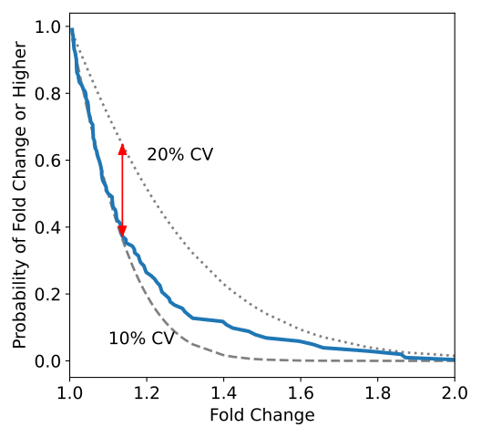
An example of this curve is show below for the probe 2682-68 in blue. The theoretical curves for a CV of 10% and 20% are also shown.
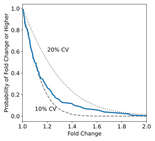
Since the above can be transformed into a CDF, Candia et al. posited that they could use the Komolgorov-Smirnov test to find a CV that gave a close theoretical distibrution. While the p-value from this test is not super meaningful, the test statistic could be used as a loss function. Here, it can be interpreted as the max absolute deviation between the theoretical curve and the empirical curve. This is shown below by the red double arrow for the 20% CV curve. Performing the KS test on a grid search of theoretical distributions gives us the ability to find the CV that achieves the minimum score.
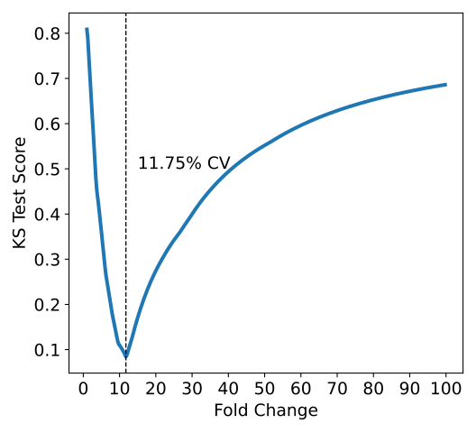
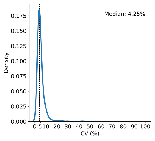
Applying this grid search to all of the probes is a bit time consuming, so I cut it down to just the first 2000. The median CV comes out around 4.25%, which is very close to the 4.5% reported by Candia et al.
CV on paired samples (via maximum-likelihood)
I believe there are much easier ways to obtain an estimate of the CV from this data that don’t involve a computationally expensive grid search. One these methods is a maximum likelihood estimate that I detailed in a previous post.
$$ CV_{mle} = 100*\sqrt{\exp\left( \frac{1}{2N} \sum z_i^{2} \right) - 1} $$
where the $z_i$ represent the absolute log fold changes, i.e. $z_i = \left| \log(y_i) - \log(x_i) \right|$.
Looking back at our probe 2682-68, we can compare the behavior of the MLE estimate to the KS test. The MLE estimate is 15.0% CV, which seems to balance out error between the beginning and end of the distribtuion. The KS test CV at 11.75% on the otherhand seems to focus on reducing error early in the distribution.
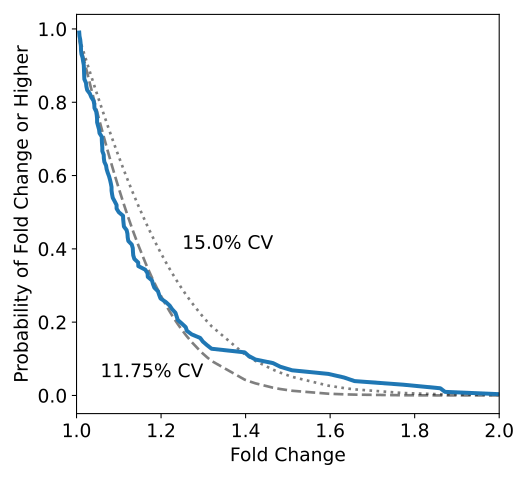
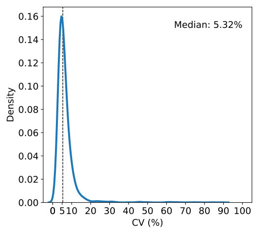
Applying this estimate to the same 2000 probes above, we get a median CV of 5.32%. This is higher than the Candia et al. estimate, but still quite good for patient samples.
- [1] Candia J, Daya GN, Tanaka T, Ferrucci L, and Walker KA (2022). Assessment of variability in the plasma 7k SomaScan proteomics assay. Scientific Reports, 12:17147. DOI: 10.1038/s41598-022-22116-0
- [2] Reed GF, Lynn F, and Meade BD (2002). Use of Coefficient of Variation in Assessing Variability of Quantitative Assays. Clinical and Diagnostic Laboratory Immunology, 1235-1239. DOI: 10.1128/cdli.9.6.1235-1239.2002