Background
A well cited paper from 2002 by Reed et al. [1] gives a link between a pair of measurments $X$ and $Y$ from a log-normal distribution and the CV of the distribution $\theta$ expressed as a decimal (as opposed to the percentage we usually use in analytical chemistry).
They note that for a given $k > 1$, the probability that $Y/X \ge k$ or $X/Y \ge k$ can be expressed by the following probability,
$$ P(Y/X \ge k\ or\ X/Y \ge k) = 2P(Y/X \ge k) = 2\Phi \left[ \frac{-\log(k)}{\sqrt{2\log(\theta^{2} + 1)}} \right], \quad k > 1 $$
where $\Phi$ is the standard normal cumulative distribution.
Re-writing the distribution
Since $X$ and $Y$ are log-normal, then $\log(X)$ and $\log(Y)$ are normally distributed and $Z = \left| \log(Y) - \log(X) \right|$ must be half normal. We can see this a bit better if we write the CDF for $Z$ and then differentiate. This is a continuous distribution so $P(Z = z) = 0$ and we can use the above equation to get the CDF of $Z$
$$ P(Z \le z) = 1 - P(Z \ge z) = 1 - P(\left| \log(Y/X) \right| \ge z) $$ $$ = 1-P(Y/X \ge e^z\ or\ X/Y \ge e^z) $$ $$ = 1 - 2\Phi \left[ \frac{-\log(e^z)}{\sqrt{2\log(\theta^{2} + 1)}} \right] $$ $$ = 1 - 2\Phi \left[ \frac{-z}{\sqrt{2\log(\theta^{2} + 1)}} \right], \quad z > 0 $$
Letting $u=-z/\sqrt{2\log(\theta^{2} + 1)}$ and differentiating with respect to $z$ gives the half-normal distribution PDF,
$$ f(z) = \frac{d}{dz}P(Z \le z) $$ $$ = \frac{d}{dz}\left[1 - 2\Phi \left[ \frac{-z}{\sqrt{2\log(\theta^{2} + 1)}} \right] \right] $$ $$ = \frac{d}{dz}\left[1 - 2\Phi[u] \right] $$ $$ = -2 \frac{1}{\sqrt{2\pi}} \exp\left(\frac{-u^2}{2}\right) \frac{d}{dz} u $$ $$ = -2 \frac{1}{\sqrt{2\pi}} \exp\left(\frac{-z^2}{2(2\log(\theta^{2} + 1))}\right) \frac{-1}{\sqrt{2\log(\theta^{2} + 1)}} $$ $$ = \frac{\sqrt{2}}{\sqrt{\pi} \sqrt{2\log(\theta^{2} + 1)}} \exp\left(\frac{-z^2}{4\log(\theta^{2} + 1)}\right), \quad z > 0 $$
The maximum likelihood estimator of $\theta$
The half-normal distribution is usually parameterized by a dispersion term $\sigma$ (which in this case is a bit different that the standard deviation). In the above expression $\sigma = \sqrt{2\log(\theta^{2} + 1)}$ which can be re-written to give a tranformation from $\sigma$ to $\theta$.
$$ \theta = f(\sigma) = \sqrt{\exp\left( \frac{1}{2} \sigma^2 \right) - 1} $$
For $\sigma$, a maximum likelihood estimator exists and has the following form for a sample of $z_1,\ …\ ,z_N$ absolute log fold changes.
$$ \hat{\sigma}_{mle} = \sqrt{\frac{1}{N}\sum z_i^{2}} $$
Due to the properties of the maximum likelihood estimator, we can use $f(\sigma)$ and $\hat{\sigma}_{mle}$ to get the maximum likelihood estimator of $\theta$.
$$ \hat{\theta}_{mle} = f(\hat{\sigma}_{mle}) = \sqrt{\exp\left( \frac{1}{2N} \sum z_i^{2} \right) - 1} $$
NOTE: Remember the two critical transformations here. First, remember $z_i$ is the absolute natural log of the fold change, i.e. $z_i = \left| \log(y_i) - \log(x_i) \right|$. Second, remember to multiply the estimate by a factor of 100 to get the CV on the standard scale, i.e. $CV = 100\ \theta$.
Monte carlo simulations
I ran a couple of quick simulations to show that this estimator gets us exactly what we are looking for. In the first simulation, I performed 2 draws of 10 and 100 samples from a log-normal distribution with progressively increasing CVs. The mean of the underlying normal distribution was kept at 10, which is reasonable for things like mass spectrometry. With the first draw, I calculated the “Classic CV Estimate”, i.e. the standard deviation divided by mean. Then I calculated the “Paired CV Estimate” using the equation above. In each case I performed 1000 repetitions.
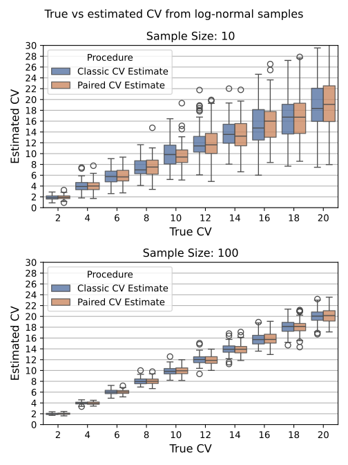
Looking at the plot above, it is clear that both estimates are getting fairly close to the true CV. In fact, once we are at 100 samples, the bias and variance of the estimators are both very low.
Where the estimator really comes in handy is when there is both random variation in the underlying variable being measured and technical variation. Think of a protein being measured in patient blood samples where every patient has a baseline expression value for that protein. In this second simulation, instead of keeping the mean of the underlying distribution at 10, I first added a small bit of noise to that mean for each pair of measurements. Therefore, 2 measurements were taken with $\mu_i = 10 + 0.1\zeta_i$, where $\zeta_i$ wass draw from the standard normal distribution.
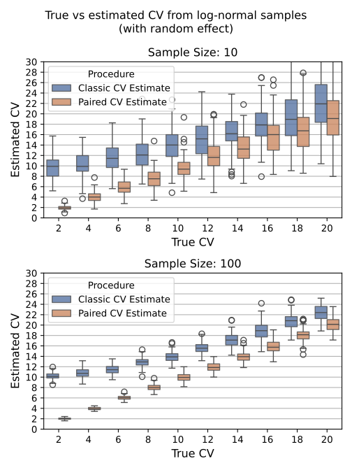
Immediately we can see that the classic CV estimate just doesn’t attempt to take into account the 2 components of the variance. The paired CV estimate, on the other hand, is able to regress out the effect coming from the $\zeta_i$s.
- [1] Reed GF, Lynn F, and Meade BD (2002). Use of Coefficient of Variation in Assessing Variability of Quantitative Assays. Clinical and Diagnostic Laboratory Immunology, 1235-1239. DOI: 10.1128/cdli.9.6.1235-1239.2002